引入包并做初始设置
from __future__ import division
from numpy.random import randn
import numpy as np
import matplotlib.pyplot as plt
plt.rc('figure', figsize=(12, 5))
np.set_printoptions(precision=4)
%pwd
通过命令查看数据文件
!head -n 10 names/yob1880.txt
通过pandas导入数据文件,并查看数据
import pandas as pd
names1880 = pd.read_csv('names/yob1880.txt', names=['name', 'sex', 'births'])
names1880
以sex分组,统计births
names1880.groupby('sex').births.sum()
合并众多数据文件,导入到同一个DataFrame
# 2010 is the last available year right now
years = range(1880, 2011)

pieces = []
columns = ['name', 'sex', 'births']

for year in years:
    path = 'names/yob%d.txt' % year
    frame = pd.read_csv(path, names=columns)

    frame['year'] = year
    pieces.append(frame)

# Concatenate everything into a single DataFrame
names = pd.concat(pieces, ignore_index=True)
concat默认是按行将DataFrame组合到一起,由于并不希望保留read_csv返回的原始行号,因此指定ignore_index=True
数据聚合
通过pivot_table对数据进行聚合,统计不同年份、不同性别的出生数
total_births = names.pivot_table('births', index='year',
                                 columns='sex', aggfunc=sum)
total_births.tail()
以sex,year分组,添加新项prop,计算指定名字的婴儿在总出生的比例。由于births是整数,因此需要在计算时将其转换为浮点数。
def add_prop(group):
    # Integer division floors
    births = group.births.astype(float)

    group['prop'] = births / births.sum()
    return group
names = names.groupby(['year', 'sex']).apply(add_prop)
names
对分组处理做有效性检查,验证prop总和是否为1.由于prop是浮点型,可以使用np.allclose检查分组总计值是否足够近似于1
np.allclose(names.groupby(['year', 'sex']).prop.sum(), 1)
为便于进一步分析,可以选取数据的一个子集:每对sex/year组合的前1000个名字
def get_top1000(group):
    return group.sort_index(by='births', ascending=False)[:1000]
grouped = names.groupby(['year', 'sex'])
top1000 = grouped.apply(get_top1000)
或者是使用手动方式
pieces = []
for year, group in names.groupby(['year', 'sex']):
    pieces.append(group.sort_index(by='births', ascending=False)[:1000])
top1000 = pd.concat(pieces, ignore_index=True)
建立索引
top1000.index = np.arange(len(top1000))
查看数据
top1000
分析命名趋势
将前1000个名字分为男女两部分
boys = top1000[top1000.sex == 'M']
girls = top1000[top1000.sex == 'F']
生成一张按year和name统计的总出生数透视表
total_births = top1000.pivot_table('births', index='year', columns='name',
                                   aggfunc=sum)
total_births
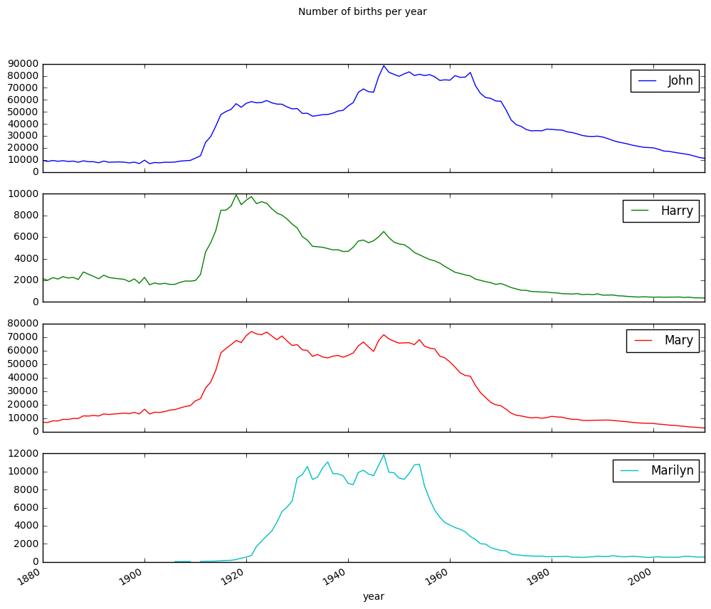
绘制'John', 'Harry', 'Mary', 'Marilyn'四个名字的曲线图
subset = total_births[['John', 'Harry', 'Mary', 'Marilyn']]
subset.plot(subplots=True, figsize=(12, 10), grid=False,
            title="Number of births per year")
plt.show()
评估命名多样性的增长
上图反映的降低情况可能意味着父母不太愿意给小孩起常见名字。
验证这个假设的方式是计算最流行的1000个名字所占的比例。
plt.figure()
table = top1000.pivot_table('prop', index='year',
                            columns='sex', aggfunc=sum)
table.plot(title='Sum of table1000.prop by year and sex',
           yticks=np.linspace(0, 1.2, 13), xticks=range(1880, 2020, 10))

plt.show()
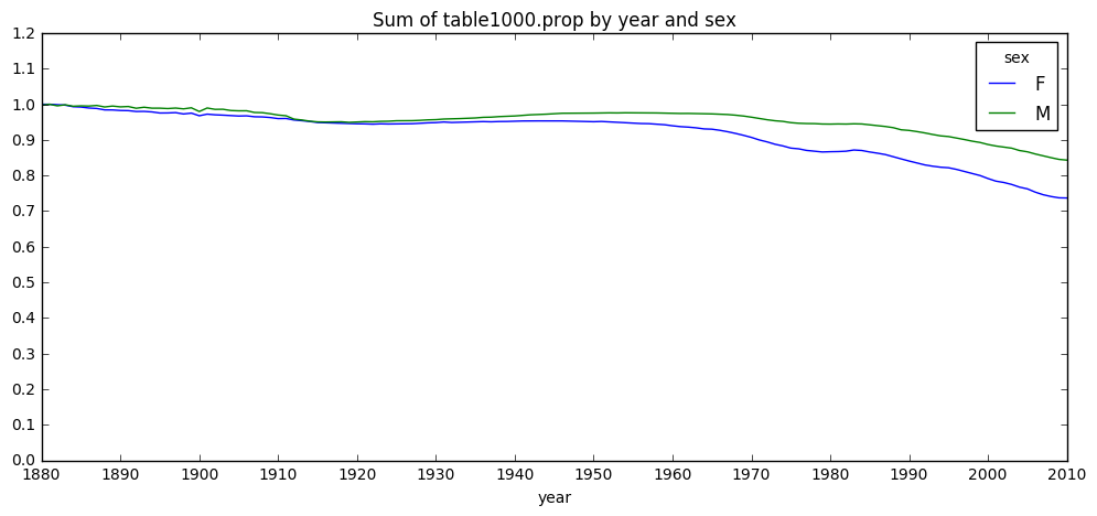
从上图可以看出,名字多样性确实出现增长,因为前1000项的比例降低。
另一种验证方式,是计算占总出生人数前50%的不同名字的数量,这里以2010年男孩的名字为例
df = boys[boys.year == 2010]
df
prop_cumsum = df.sort_index(by='prop', ascending=False).prop.cumsum()
prop_cumsum[:10]
prop_cumsum.values.searchsorted(0.5)
由于数组索引是从0开始的,因此需要给这个结果加1,这里得到的最终结果是117
拿1900年的数组做比较,这个结果要小的多
df = boys[boys.year == 1900]
in1900 = df.sort_index(by='prop', ascending=False).prop.cumsum()
in1900.values.searchsorted(0.5) + 1
现在就可以对所有的year/sex组合执行上述计算
def get_quantile_count(group, q=0.5):
    group = group.sort_index(by='prop', ascending=False)
    return group.prop.cumsum().values.searchsorted(q) + 1

diversity = top1000.groupby(['year', 'sex']).apply(get_quantile_count)
diversity = diversity.unstack('sex')
绘制多样性图表
diversity.plot(title="Number of popular names in top 50%")
plt.show()
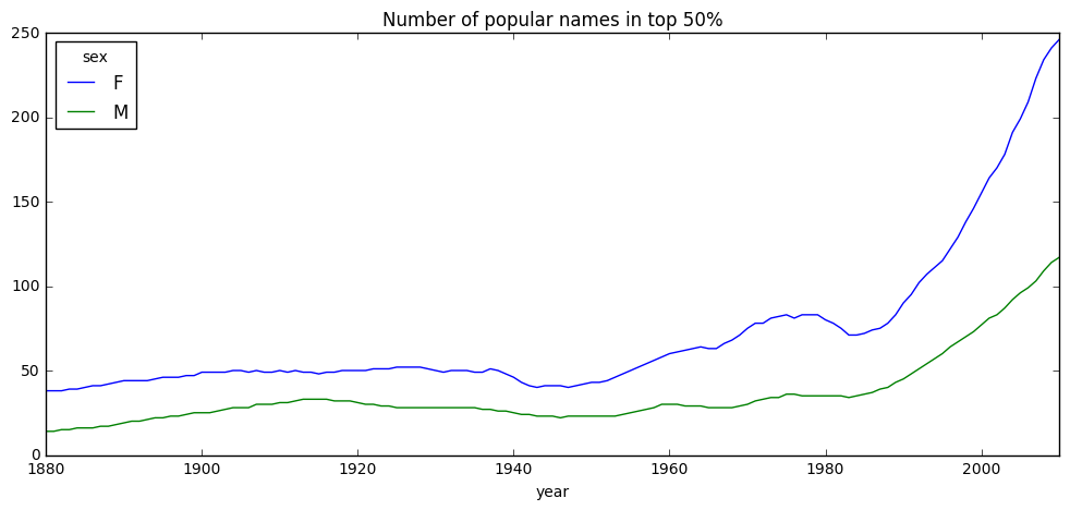
由图上我们可以看出,女孩的名字多样性要高于男孩,而且越来越高。
“最后一个字母”的变革
这里有一个研究:近百年来,男孩名字在最后一个字母上的分布发生显著变化。
为验证这个研究,首先对全部数组在年度、性别以及末尾字母进行聚合。
# extract last letter from name column
get_last_letter = lambda x: x[-1]
last_letters = names.name.map(get_last_letter)
last_letters.name = 'last_letter'

table = names.pivot_table('births', index=last_letters,
                          columns=['sex', 'year'], aggfunc=sum)
选出具有一定代表性的三年,输出前面几行
subtable = table.reindex(columns=[1910, 1960, 2010], level='year')
subtable.head()
对数据表进行规范化处理,计算出各性别各末尾字母所占总出生人数比例
subtable.sum()
letter_prop = subtable / subtable.sum().astype(float)
绘制各年度个性别条形图
import matplotlib.pyplot as plt

fig, axes = plt.subplots(2, 1, figsize=(10, 8))
letter_prop['M'].plot(kind='bar', rot=0, ax=axes[0], title='Male')
letter_prop['F'].plot(kind='bar', rot=0, ax=axes[1], title='Female',
                      legend=False)
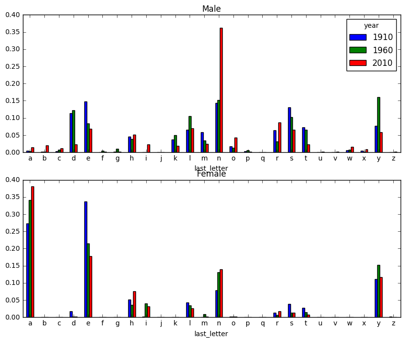
从图上可知,以n结尾的男孩名字显著增长。
对完整的表进行上面的处理
letter_prop = table / table.sum().astype(float)
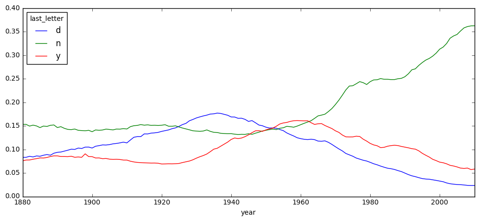
dny_ts = letter_prop.ix[['d', 'n', 'y'], 'M'].T
dny_ts.head()
变成女孩子的男孩子名(相反)
另一个趋势是,早年流行于男孩的名字,现在被女孩子使用。
在top1000数据集,查找以“lesl”开头的名字
all_names = top1000.name.unique()
mask = np.array(['lesl' in x.lower() for x in all_names])
lesley_like = all_names[mask]
lesley_like
利用这个结果过滤其他名字,并按名字分组计算出生数及相对频率
filtered = top1000[top1000.name.isin(lesley_like)]
filtered.groupby('name').births.sum()
按性别和年度进行聚合,并按年度进行规范化处理
table = filtered.pivot_table('births', index='year',
                             columns='sex', aggfunc='sum')
table = table.div(table.sum(1), axis=0)
table.tail()
绘制性别-年度曲线
table.plot(style={'M': 'k-', 'F': 'k--'})
